Sorting Algorithms

Sorting

In one of the previous posts, we have discussed 'Binary search' in some detail. One of the requirements to run a Binary Search is that the data in our Array is sorted. In this blog, let's take a look at different ways to sort the lists and find the best way to sort the list.

1. Bubble sort

Figure [1] Bubble Sort

Here's the code for bubble sorting a simple array:

def bubble_sort(array):

    n = len(array)

    for i in range(n):

        already_sorted = True

        for j in range(n-i-1):

            if array[j] > array[j+1]:

                array[j], array[j+1] = array[j+1], array[j]

            already_sorted = False

        if already_sorted:

            break

    return array

print(bubble_sort([2,3,9,8,7,1]))

Since the bubble sort algorithm has 2 for loops, it has a time complexity of O(n^2).

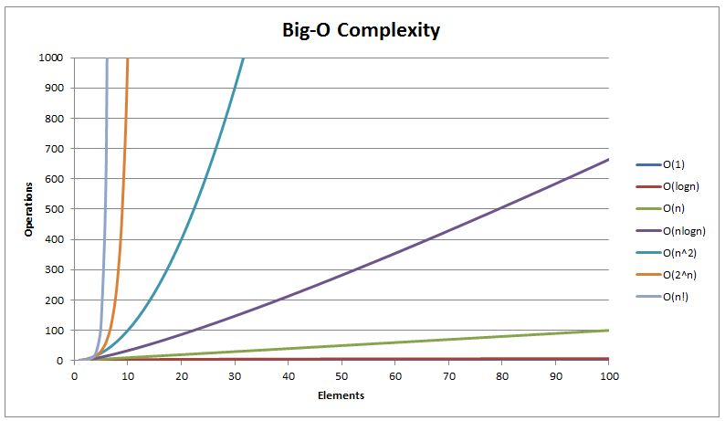Figure [2] Time Complexities Graph

Based off the graph in Figure 2, we can see that the sorting algorithm has a less desirable time complexity.

2. Insertion sort

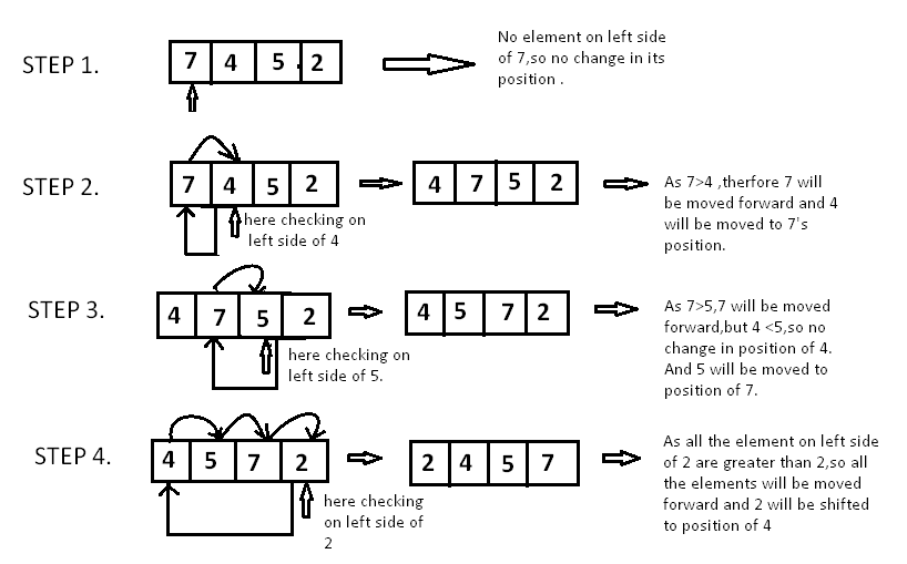Figure [3] Insertion Sort

Here's the code for implementing insertion sort:

def insertion_sort(array):

    for i in range(1, len(array)):

        key_item = array[i]

        

        j = i-1

        while j>=0 and array[j] > key_item:

            array[j+1] = array[j]

            j-=1

        

        array[j+1] = key_item

    return(array)

print(insertion_sort([2,3,9,8,7,1]))

Despite having a better inner loop efficiency as compared to bubble sort, insertion sort still has 2 loops and thus, has a time complexity of O(n^2).

3. Merge sort

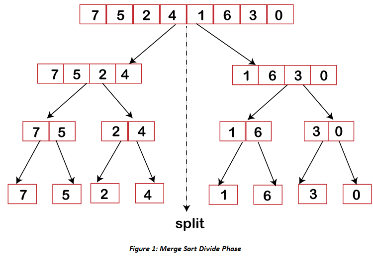Figure [4] Merge Sort

Here's the code for implementing merge sort: 

def merge(left, right):

    if len(left) == 0:

        return right

    if len(right) == 0:

        return left

    result = []

    index_left = index_right = 0

    while len(result) < len(left) + len(right):

        if left[index_left] <= right[index_right]:

            result.append(left[index_left])

            index_left += 1

        else:

            result.append(right[index_right])

            index_right += 1

        if index_right == len(right):

            result += left[index_left:]

            break

        if index_left == len(left):

            result += right[index_right:]

            break

    return result

def merge_sort(array):

    if len(array) < 2:

        return array

    midpoint = len(array) // 2

    return merge(

        left=merge_sort(array[:midpoint]),

        right=merge_sort(array[midpoint:]))

print(merge_sort([2,3,9,8,7,1]))

While it is a little hard to comprehend what is happening in a merge sort from the code at first glance, its actually quite simple. 

One of the concepts that we need to understand is that of 'Divide & Conquer' which itself is based on recursion.

There are 2 parts to the code above, the first is recursively splitting the input into half and the second is the merging both halves to produce a sorted array.

Time complexity of the Merge sort algorithm is 'O(n*log2n)' which makes it much more efficient than either bubble or insertion sorts but the downside is that merge sort uses a lot more memory and thus is to be avoided when working with a large list/array.

4. Quick sort

In quick sort, you partition the array into 2 sub-arrays after selecting a pivot, all the elements smaller than the pivot go into one of the arrays and all elements larger than the pivot go into the other array.

def quicksort(array):

    if len(array) < 2:

        return array

    low, same, high = [], [], []

    pivot = array[randint(0, len(array) - 1)]

    for item in array:

        if item < pivot:

            low.append(item)

        elif item == pivot:

            same.append(item)

        elif item > pivot:

            high.append(item)

    return quicksort(low) + same + quicksort(high)

print(quicksort([2,3,9,8,7,1]))

Time complexity of the Quicksort algorithm is 'O(n*log2n)' which is the same as Merge Sort.

Quicksort is used to overcome the space inefficiencies of merge sort. Here's how it works:

1. If the list is empty or just has one element, we return it since there is no sorting involved.

2. We pick a random element from the list and set it as our 'pivot'.

3. We perform a partitioning operation, we set all elements less than the pivot in a separate array, then all elements equal to the pivot in another array, and then all elements larger than the pivot in a third array.

4. The pivot element divides the array into 2 parts which can then be sorted independently by recursively calling the quicksort.

4. Timsort sort

Figure [5] Timsort = Insertion sort + merge sort

Timsort is based on 'insertion sort' and 'merge sort'. Used in Python's sort() and sorted() methods.

In Timsort, we first sort small pieces using Insertion Sort, then merges the pieces using a merge of merge sort. The implementation of Timsort is quite complicated, please refer to this article if you're looking for more information on this topic.

Timsort has a worst case complexity of O(n*log(n)) as well.

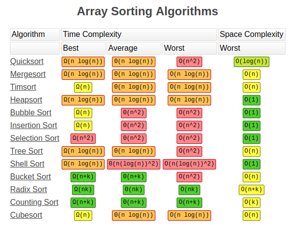
In summary, let's take a look at the different sorting methods and their time/space complexities.

Thank you for reading! 

---

References:

[1] https://realpython.com/sorting-algorithms-python/

[2] https://www.geeksforgeeks.org/timsort/

[3] https://jovian.ai/learn/data-structures-and-algorithms-in-python/lesson/lesson-3-sorting-algorithms-and-divide-and-conquer

[4] https://www.geeksforgeeks.org/timsort/